The previous sections dealt with the dynamics of any spin system, but most of the work during my PhD studies only concern radical pairs. This section is, therefore, restricted to the discussion of radical pairs. An introduction to radical pair dynamics and the important concept of singlet-triplet mixing may be found in the supporting information of my paper Towards predicting intracellular radiofrequency radiation effects.
Quantum yields
The reaction operators describe how the radical pair ensemble may be diminished (or enlarged) over time, as various processes may, for example, turn the radical pair into different chemical species. When multiple processes are possible it is often desirable to know the amount of radical pairs that participate in each process, and this is described by the so-called quantum yields. A reaction operator specifies both the subspace of the spin system that reacts, described by a projection operator \(\require{newcommand} \newcommand{\vc}[1]{\mathbf{#1}} \newcommand{\desc}[1]{\begin{quote}\emph{#1}\end{quote}} \newcommand{\p}{\partial} \newcommand{\bra}[1]{\langle #1 |\,} \newcommand{\ket}[1]{\,| #1 \rangle} \newcommand{\braket}[2]{\langle #1 | #2 \rangle} \newcommand{\matel}[3]{\langle #1 | #2 | #3 \rangle} \newcommand{\mexp}[1]{\langle #1 \rangle} \newcommand{\kb}[2]{| #1 \rangle\langle #2 |} \DeclareMathOperator{\Tr}{Tr} \vc{P}\), as well as a rate constant \(k\), and the quantum yield may be derived by noting that an amount of radical pairs \(k\Tr(\vc{P}\rho(t))\) reacts through this particular reaction pathway at time instance \(t\). Thus the quantum yield is defined as the accumulated amount of radical pairs reacting through the reaction pathway:
\begin{equation} \phi = k\int_0^\infty\Tr(\vc{P}\rho(t)) \, dt \, . \label{eq_quantumyield_definition} \end{equation}Note that this definition is only useful if there are no processes that create more radical pairs, unless a specific and finite time-interval is considered. When there are processes that create radical pairs at a constant rate one might look for a steady-state solution to the Liouville-von Neumann equation instead, i.e. setting \(\frac{d\rho}{dt} = \vc{0}\).
Liouville space
Since the density operator is itself an operator, anything that "operates on the operator" is called a superoperator; i.e. a superoperator is a mathematical object that operates on an operator rather than a state vector. In particular, the commutator with \(\vc{H}\) and anti-commutators with projection operators are examples of superoperators:
\begin{equation} \vc{H}^\times(\, \cdot \,) = [\vc{H},\,\cdot\,], \qquad \vc{K}_i^\times(\, \cdot \,) = \{\vc{P}_i,\,\cdot\,\}, \end{equation}where \(^\times\) denotes a superoperator. Note that a reaction operator of the Haberkorn type is assumed here for the sake of a concrete example. Thus the Liouville-von Neumann equation can be written as:
\begin{equation} \frac{d\rho}{dt} = -\frac{i}{\hbar}\vc{H}^\times(\rho) + \frac{k}{2}\vc{K}^\times(\rho) \, . \end{equation}Note how the superoperators act on \(\rho\) both from the left and the right; i.e. both on the row and column space of \(\rho\). This motivates the introduction of the superoperator space or Liouville space, which is a much larger Hilbert space that so to speak "separates the row and column spaces of \(\rho\)". This is done by turning \(\rho\) into the superoperator space state vector \(\vec{\rho}\), which is obtained by "reshaping" \(\rho\) from an \(n \times n\) matrix to a vector in an \(n^2\)-dimensional Hilbert space:
\begin{equation} \vec{\rho}_{i+nj} = \rho_{i,j} \, . \end{equation}Similarly the superoperators have a different form in the super space, as defined by the following example:
\begin{equation} \vc{A}^\times(\rho) = \vc{T} \rho \vc{R} \quad \rightarrow \quad \vc{A}^\times \vec{\rho} = \vc{T} \otimes \vc{R}^T \, \vec{\rho} , \end{equation}where \(\otimes\) is the Kronecker tensor product and \(\vc{A}^\times\) becomes and \(n^2 \times n^2\) matrix. Note that the transpose of the right-side operator \(\vc{R}\) is used rather than the hermitian conjugate (even for complex operators). The Hamiltonian superoperator can then be written as:
\begin{equation} \vc{H}^\times = \vc{H} \otimes \vc{1} - \vc{1} \otimes \vc{H}^T, \end{equation}and the Haberkorn reaction operator can be written in a similar way:
\begin{equation} \vc{K}_i^\times = \vc{P}_i \otimes \vc{1} + \vc{1} \otimes \vc{P}_i^T \, . \end{equation}This leads to the following form of the Liouville-von Neumann equation in Liouville space:
\begin{equation} \frac{d \vec{\rho}}{dt} = \vc{L}\vec{\rho}, \label{eq_Liouvillespace_LvN} \end{equation}where \(\vc{L} = -\frac{i}{\hbar}\vc{H}^\times + \frac{k}{2}\vc{K}^\times\) is known as the Liouvillian superoperator.
The form of Eq. (\ref{eq_Liouvillespace_LvN}) is much simpler to solve than the Liouville-von Neumann equation in the native Hilbert space with a reaction operator, although the cost of simplicity is an enlargement of the Hilbert space which becomes significant when many spins are considered.Quantum yields are also calculated much easier in Liouville space, and this may be shown using the following two properties of the Laplace transformation (the Laplace transformation is defined as \(\mathcal{L}\{f\} = \int_0^\infty e^{-st}f(t) \, dt\) and is a generalization of the Fourier transform):
\begin{equation} \mathcal{L}\left\{\frac{d\rho}{dt}\right\} = s\mathcal{L}\left\{\rho\right\} - \rho(0), \qquad \lim_{s \to 0}s\mathcal{L}\left\{\rho\right\} = \lim_{t \to \infty}\rho(t), \end{equation}which may be inserted in Eq. (\ref{eq_quantumyield_definition}) assuming \(s \to 0\):
\begin{equation} \phi = k\Tr\left(\vc{P}\int_0^\infty\rho \, dt\right) = k\Tr(\vc{P}\mathcal{L}\left\{\rho\right\}) = -k\Tr\left(\vc{P}\vc{L}^{-1}\left(\rho(0)\right)\right) \, . \end{equation}Note the assumption that \(\lim_{t \to \infty}\rho(t) = \vc{0}\) and that the Liouvillian is time-independent.
The radical pair mechanism
A radical pair produced in a spin-correlated state such as the singlet or a triplet state will normally be subject to singlet-triplet mixing, which is an oscillation of the spin state between the singlet and triplet states (this is not the case if the initial singlet or triplet state is an eigenstate of the Hamiltonian as may be the case if e.g. a very strong exchange interaction is present). These oscillations may occur for all the systems in a radical pair ensemble and affect the outcome of any spin-dependent process, as described by reaction operators. The oscillation frequency, i.e. the singlet-triplet mixing rate, depends on the magnetic interactions in the radical pair ensemble, and in particular it depends on any external magnetic field - both stationary fields such as the geomagnetic field, or oscillating fields from electromagnetic radiation. Consider the simple reaction scheme in Fig. 1A which has two spin-dependent reaction pathways, a singlet reaction and a triplet reaction.
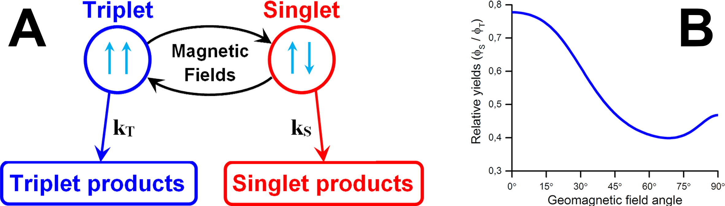
Figure 1 - The radical pair mechanism.
A: A simple reaction scheme.
A radical pair may be created in a spin-correlated state (singlet or triplet), and magnetic interactions drive singlet-triplet mixing and thereby affect the amounts of singlet and triplet quantum yields.
An external magnetic field such as the geomagnetic field or magnetic component of radiation may affect the mixing and hence affect the relative yields.
B: Effect on the relative quantum yield of rotating the external magnetic field from the \(z\)-axis (\(0^\circ\)) towards the \(x\)-axis (\(90^\circ\)) in the \(xz\)-plane for a model radical pair.
The quantum yields of these two reaction pathways are given by:
\begin{equation} \phi_S = k_S\int_0^\infty\Tr(\vc{P}_S\rho)\, dt, \qquad \phi_T = k_T\int_0^\infty\Tr(\vc{P}_T\rho)\, dt, \end{equation}where the rate constants \(k_S\) and \(k_T\) may be different, and the singlet and triplet subspace projections are given by:
\begin{equation} \vc{P}_S = \frac{1}{4}\vc{1} - \vc{S}_1 \cdot \vc{S}_2, \qquad \vc{P}_T = \frac{3}{4}\vc{1} + \vc{S}_1 \cdot \vc{S}_2, \end{equation}where \(\vc{S}_1\) and \(\vc{S}_2\) are the spin operators for the two unpaired electronic spins of the radical pair. Note that the quantum yields should be normalized to sum up to unity:
\begin{equation} \Phi_S = \frac{\phi_S}{\phi_S + \phi_T}, \qquad \Phi_T = \frac{\phi_T}{\phi_S + \phi_T} \, . \end{equation}Here \(\Phi_S\) and \(\Phi_T\) are the normalized yields.
A radical pair ensemble following a reaction scheme similar to Fig. 1A, as described above, may function as a chemical compass; the orientation of an external magnetic field relative to the orientation of the radical pairs may influence the singlet-triplet mixing and thereby affect the relative amount of singlet and triplet yields. Note that this assumes that the radical pairs are constrained in some way, rather than having an ensemble of randomly oriented radical pairs.
The effect of the orientation of an external magnetic field on the quantum yields is illustrated in Fig. 1B for a simple radical pair model, but note that at least one anisotropic hyperfine interaction in the model is needed in order to define the molecular reference frame - if all internal interactions in the radical pair are isotropic the orientation of the external magnetic field has no impact on the quantum yields (due to rotational symmetry). The ability of magnetic fields to affect quantum yields through the coherent singlet-triplet mixing is the essence of the radical pair mechanism.
Efficient calculation of quantum yields
Once a few assumptions may be applied it becomes significantly easier to solve the Liouville-von Neumann equation, and the first assumption is that only a single spin-independent reaction pathway exists, corresponding to Fig. 1A for the case \(k = k_S = k_T\). Inserting the general solution to the Liouville-von Neumann equation into the equation describing the quantum yield, Eq. (\ref{eq_quantumyield_definition}), one obtains:
\begin{align} \phi &= k\int_0^\infty\Tr\left(\vc{P}\exp\left(-\frac{i}{\hbar}\vc{H}t\right) \rho(0) \exp\left(\frac{i}{\hbar}\vc{H}t\right)\right) f(t) \, dt, \\ &= k\sum_n\sum_m\matel{m}{\vc{P}}{n}\matel{n}{\rho(0)}{m} \int_0^\infty e^{-i(\omega_n - \omega_m)t} f(t) \, dt, \end{align}where \(f(t)\) is a decay function. In particular an exponential decay model is assumed. The two parts of the sum where \(n>m\) and \(n<m\) are complex conjugates of each other, but the matrix elements are real. Thus by relabelling \(n \leftrightarrow m\) for the case \(n<m\), the equation may be rewritten as:
\begin{equation} \phi = k\sum_{n > m} \vc{P}_{mn} [\rho(0)]_{nm} \int_0^\infty\left( e^{-i\omega_{nm}t} + e^{i\omega_{nm}t} \right) f(t) \, dt + k\sum_n \vc{P}_{nn}[\rho(0)]_{nn} \int_0^\infty f(t) \, dt, \end{equation}where \(\vc{P}_{mn} = \matel{m}{\vc{P}}{n}\), \([\rho(0)]_{nm} = \matel{n}{\rho(0)}{m}\) and \(\omega_{nm} = \omega_n - \omega_m\). It is evident that the integral is the Fourier transform of \(f\) which for the exponential model is:
\begin{equation} \int_{-\infty}^\infty e^{-i\omega_{nm}t} e^{-k|t|} \, dt = \frac{k}{k^2 + \omega_{nm}^2} \, . \end{equation}The final expression is therefore:
\begin{equation} \phi = \sum_{n=1}^N\sum_{m=1}^N\matel{m}{\vc{P}}{n}\bra{n} \rho(0) \ket{m} \frac{k^2}{k^2 + (\omega_n - \omega_m)^2} \, . \label{eq_basicspindyn_solverSymmetricDecay} \end{equation}Here \(N\) is the dimension of the Hilbert space. Note that the largest contribution to the quantum yield is obtained for a radical pair with a close-packed spectrum of eigenvalues, and that degenerate eigenstates potentially contribute most.
The expression in Eq. (\ref{eq_basicspindyn_solverSymmetricDecay}) is efficient for computing quantum yields, and by neglecting terms in the sum where \(\omega_{nm}^2/k^2\) is large the computations may be even faster. Still, the dimension of the space, \(N\), scales exponentially with addition of nuclear spins, and this limitation can be somewhat mitigated by applying a slightly different method that unfortunately requires further assumptions.
If, in addition to having only spin-independent decay, one assumes that no coupling exists between the unpaired electrons of the radical pair and that the radical pair is produced in the singlet state, i.e. \(\rho(0) = \vc{P}_S/\Tr(\vc{P}_S)\), the singlet quantum yield may be written as:
\begin{align} \phi_S &= k \int_0^\infty \Tr\left( \vc{P}_S \exp\left(-\frac{i}{\hbar}\vc{H}t\right) \frac{\vc{P}_S}{\Tr(\vc{P}_S)} \exp\left(\frac{i}{\hbar}\vc{H}t\right) \right) f(t) \, dt, \\ &= k \int_0^\infty \Tr\left( \left(\frac{1}{4}\vc{1} - \vc{S}_1\cdot\vc{S}_2\right) \exp\left(-\frac{i}{\hbar}\vc{H}t\right) \frac{\frac{1}{4}\vc{1} - \vc{S}_1\cdot\vc{S}_2}{\Tr(\vc{P}_S)} \exp\left(\frac{i}{\hbar}\vc{H}t\right) \right) f(t) \, dt, \end{align}where the four elements of the trace are evaluated as:
\begin{align} \Tr\left(\frac{1}{4}\vc{1} \exp\left(-\frac{i}{\hbar}\vc{H}t\right) \frac{1}{4}\vc{1}\exp\left(\frac{i}{\hbar}\vc{H}t\right) \right) &= \frac{1}{16}\Tr(\vc{1}), \\ -\Tr\left(\vc{S}_1\cdot\vc{S}_2 \exp\left(-\frac{i}{\hbar}\vc{H}t\right) \frac{1}{4}\vc{1}\exp\left(\frac{i}{\hbar}\vc{H}t\right) \right) &= -\frac{1}{4}\Tr(\vc{S}_1\cdot\vc{S}_2), \\ -\Tr\left(\frac{1}{4}\vc{1} \exp\left(-\frac{i}{\hbar}\vc{H}t\right) \vc{S}_1\cdot\vc{S}_2\exp\left(\frac{i}{\hbar}\vc{H}t\right) \right) &= -\frac{1}{4}\Tr(\vc{S}_1\cdot\vc{S}_2),, \\ \Tr\left(\vc{S}_1\cdot\vc{S}_2 \exp\left(-\frac{i}{\hbar}\vc{H}t\right) \vc{S}_1\cdot\vc{S}_2\exp\left(\frac{i}{\hbar}\vc{H}t\right) \right) &= \vc{T}, \end{align}where:
\begin{align} \vc{T} &= \sum_{i,j} \Tr\left(\overbrace{\vc{S}_{1i} \exp\left(-\frac{i}{\hbar}\vc{H}_1 t\right) \vc{S}_{1j} \exp\left(\frac{i}{\hbar}\vc{H}_1 t\right)}^{\vc{R}^{(1)}_{ij}} \cdot \overbrace{\vc{S}_{2i} \exp\left(-\frac{i}{\hbar}\vc{H}_2 t\right) \vc{S}_{2j} \exp\left(\frac{i}{\hbar}\vc{H}_2 t\right)}^{\vc{R}^{(2)}_{ij}} \right), \\ &= \sum_{i,j} \Tr\left(\vc{R}^{(1)}_{ij} \right) \Tr\left( \vc{R}^{(2)}_{ij} \right) = \sum_{i,j} R^{(1)}_{ij} R^{(2)}_{ij}, \quad R^{(n)}_{ij} = \Tr\left(\vc{R}^{(n)}_{ij} \right) \, . \end{align}Here \(\vc{H}_1\) and \(\vc{H}_2\) are the Hamiltonians for the two subspaces, i.e. a space for each radical, and this splitting of the Hamiltonian is possible since the radicals are uncoupled. The indices \(i\) and \(j\) refer to the three components of the spin operator, \(i,j \in \{x,y,z\}\), and the superscript \({(n)}\) refers to radical 1 or radical 2. The quantity \(\Tr(\vc{S}_1 \cdot \vc{S}_2)\) may be rewritten as:
\begin{equation} \Tr(\vc{S}_1 \cdot \vc{S}_2) = \sum_n\bra{n}\left(\vc{S}_{1z}\vc{S}_{2z} + \frac{1}{2}(\vc{S}_{1+}\vc{S}_{2-} + \vc{S}_{1-}\vc{S}_{2+}) \right)\ket{n} = \sum_n\matel{n}{\vc{S}_{1z}\vc{S}_{2z}}{n}, \end{equation}where the four terms in the sum cancel such that \(\Tr(\vc{S}_1 \cdot \vc{S}_2) = 0\). The quantum yield is therefore:
\begin{align} \phi_S &= k\int_0^\infty \frac{1}{\Tr(\vc{P}_S)}\left( \frac{1}{16} \Tr{\vc{1}} + \sum_{i,j} R^{(1)}_{ij} R^{(2)}_{ij} \right) f(t) \, dt, \\ &= k\int_0^\infty \left( \frac{1}{4} + \frac{1}{\Tr(\vc{P}_S)}\sum_{i,j} R^{(1)}_{ij} R^{(2)}_{ij} \right) f(t) \, dt, \end{align}The time-dependence in \(R^{(n)}_{ij}\) is separated using completeness relations:
\begin{align} R^{(n)}_{ij} &= \sum_{p,q} \Tr\left( \vc{S}_{ni} \ket{p}\bra{p} \exp\left(-\frac{i}{\hbar}\vc{H}_n t\right) \vc{S}_{nj} \ket{q}\bra{q} \exp\left(\frac{i}{\hbar}\vc{H}_n t\right) \right), \\ &= \sum_{p,q} \matel{q}{\vc{S}_{ni}}{p} \matel{p}{\vc{S}_{nj}}{q} \, e^{-i(\omega_p - \omega_q) t}, \end{align}hence the quantum yield is given by:
\begin{equation} \phi_S = k\int_0^\infty \left( \frac{1}{4} + \sum_{i,j} \sum_{p,q,r,s} \matel{q}{\vc{S}_{1i}}{p} \matel{p}{\vc{S}_{1j}}{q}\matel{r}{\vc{S}_{2i}}{s} \matel{s}{\vc{S}_{2j}}{r} \frac{e^{-i(\omega_p - \omega_q + \omega_r - \omega_s) t}}{\Tr(\vc{P}_S)} \right) f(t) \, dt, \end{equation}Assuming an exponential decay model again results in a Fourier transform of the exponential decay function, thus providing the final equation for the quantum yield:
\begin{equation} \phi_S = \frac{1}{4} + \frac{1}{\Tr(\vc{P}_S)}\sum_{i,j} \sum_{p,q,r,s} \matel{q}{\vc{S}_{1i}}{p} \matel{p}{\vc{S}_{1j}}{q}\matel{r}{\vc{S}_{2i}}{s} \matel{s}{\vc{S}_{2j}}{r} \frac{k^2}{k^2 + (\omega_p - \omega_q + \omega_r - \omega_s)^2} \, . \label{eq_basicspindyn_solverRPSymUncoupled} \end{equation}Eq. (\ref{eq_basicspindyn_solverRPSymUncoupled}) is quite similar to Eq. (\ref{eq_basicspindyn_solverSymmetricDecay}), but splitting the Hilbert space into two smaller spaces may have a significant effect on the computational performance once the methods are implemented. Adding a magnetic nucleus only scales one of the two smaller spaces for the method in Eq. (\ref{eq_basicspindyn_solverRPSymUncoupled}) whereas it would scale the total space in the method described by Eq. (\ref{eq_basicspindyn_solverSymmetricDecay}).